Showing posts with label programming. Show all posts

How to create banner in bash


Install figlet

  
sudo apt update
sudo apt install figlet
    
figlet is a fun command-line tool that turns regular text into large ASCII art-style letters. It’s mostly used for decoration in terminal scripts, welcome messages, or just to make things look cooler in the shell.

Bash Code

  
#!/bin/bash
# Define colors for printouts
GREEN="\033[1;32m"
BLUE="\033[1;34m"
YELLOW="\033[1;33m"
RESET="\033[0m"
CYAN="\033[1;36m"
MAGENTA="\033[1;35m"

# Impressive entry dialog
clear
echo -e "${BLUE}"
figlet -c 'PARKLIZE'
echo -e "${RESET}"
sleep 3  # Pause for a few seconds to allow the user to read the banner
    

How to check all available Java versions on Linux

In order to check the list of Java versions available on our Linux machine, we can use the following command.


$ sudo update-alternatives --config java


 Selection    Path                                            Priority   Status

------------------------------------------------------------

  0            /usr/lib/jvm/java-17-openjdk-amd64/bin/java      1711      auto mode

  1            /usr/lib/jvm/java-11-openjdk-amd64/bin/java      1111      manual mode

* 2            /usr/lib/jvm/java-17-openjdk-amd64/bin/java      1711      manual mode

  3            /usr/lib/jvm/java-8-openjdk-amd64/jre/bin/java   1081      manual mode


The one with * indicates the current version. We can check the current Java version being used directly as well.


$ java --version

openjdk 17.0.10 2024-01-16
OpenJDK Runtime Environment (build 17.0.10+7-Ubuntu-122.04.1)
OpenJDK 64-Bit Server VM (build 17.0.10+7-Ubuntu-122.04.1, mixed mode, sharing)

Setting up Jena Fuseki using Docker image

 Apache Jena is a free and open source Java framework for building Semantic Web and Linked Data applications. The framework is composed of different APIs interacting together to process RDF data, as we can see from the figure below.

The focus of this post is about setting up Fuseki using Docker. In short, Fuseki a SPARQL server which can present RDF data and answer SPARQL queries over HTTP. 

The content of this post is as follows:

  • Run Fuseki server with Docker image
  • Configuration of Fuseki data service
  • Test SPARQL queries on the server using cURL


Run Fuseki server with Docker image

If you are familiar with Docker, it is very convinient to set up a Fuseki server using a Fuseki Docker image from the Docker Hub, which is a cloud-based repository service provided by Docker for finding, storing, and sharing container images. 

I have Docker Desktop in my laptop which provides an integrated development environment (IDE) for building, shipping, and running containerized applications using Docker. 

After pulling the Fuseki Docker image, we can follow the instruction to run a Fuseki server already:


docker run --rm -it -p 3030:3030 --name fuseki -e ADMIN_PASSWORD=[PASSWORD] -e ENABLE_DATA_WRITE=[true|false] -e ENABLE_UPDATE=[true|false] -e QUERY_TIMEOUT=[number in milliseconds] --mount type=bind,source="$(pwd)"/fuseki-data,target=/fuseki-base/databases secoresearch/fuseki

The server should be accessible at http://localhost:3030.


Configuration of Fuseki data service

So far so good. One thing to note is that Fuseki server is running with default settings or configurations. According to the instruction in the Fuseki Docker image page, it also mentioned that we need to add configuration file assembler.ttl file under the fuseki-configuration/ folder. You can find the ttl file on the GitHub repo of the Fuseki Docker image provider. The instruction to run the Fuseki server with custom configuration is as follows:


mkdir fuseki-data
mkdir fuseki-configuration
cp -p assembler.ttl fuseki-configuration/
# edit fuseki-configuration/assembler.ttl to enable the endpoints you wish
docker run --rm -it -p 3030:3030 --name fuseki -e ADMIN_PASSWORD=[PASSWORD] -e QUERY_TIMEOUT=[number in milliseconds] --mount type=bind,source="$(pwd)"/fuseki-data,target=/fuseki-base/databases --mount type=bind,source="$(pwd)"/fuseki-configuration,target=/fuseki-base/configuration secoresearch/fuseki
Otherwise, we can also come up with our own configuration file based on the Fuseki Data Service Configuration Syntax. For example, in my case, I would like to simply test with some dummy RDF data loaded when the server starting up, so I also set up a MemoryModel for a .ttl file containing the RDF data I'm interested in. Everytime the server is starting, it contains the RDF dataset that I can play around with, and run some SPARQL queries over the dataset.


<#service> rdf:type fuseki:Service ;
    fuseki:name              "ds" ;   # http://host:port/ds
    fuseki:dataset           <#tdb> ;
    fuseki:endpoint [ 
         # SPARQL query service
        fuseki:operation fuseki:query ; 
        fuseki:name "sparql"
    ] ;
    
    ... ...
        
<#tdb>    rdf:type ja:RDFDataset ;
    rdfs:label "EnergyConsumption" ;
    ja:defaultGraph
      [ rdfs:label "DAYTON.ttl" ;
        a ja:MemoryModel ;
        ja:content [ja:externalContent <ttl file location>] ;
      ] ;
    .

Test SPARQL queries on the server 

If you are planning to interact with the Fuseki server set up in your program such as using Python, you might need to test SPARQL queries via HTTP out first. One way is directly using the browser and type your endpoint with your query parameter:


http://localhost:3030/ds/sparql?query=SELECT%20*%20WHERE%20{?s%20?p%20?o}%20limit%203

If you are using curl for testing a SPARQL query, you can submit a URL-encoded SPARQL query 


curl "http://localhost:3030/ds/sparql?query=SELECT%20*%20WHERE%20\{?s%20?p%20?o\}%20limit%203"

It seems escapes for starting and ending brackets are needed. For more details regarding using curl for SPARQL queries, one can refern to cURLing SPARQL, which contains much more details regarding the topic.

How to use the OpenAPI code generator with your OpenAPI specification for your REST API implementation

In this post, we will introduce what is the OpenAPI code generator, and what it does in the context of the REST API and OpenAPI specification. Although I had a clear understanding of the REST API and why we need follow OpenAPI specification, it was not so clear at the beginning when it comes to the OpenAPI code generator and what it generates, and how it helps. If you have the same confusion, you are in the right place.

The content is as follows:
  • Background
  • Install OpenAPI code generator
  • Prepare OpenAPI specification - YAML/JSON file
  • Generate server stub using the OpenAPI code generator
  • Implement your functionality on top of the generated server sub

Background

Before delving into OpenAPI code generator, let's first talk about some background of the OpenAPI specification first. 

It comes from the API-first design or top-down API development where we specify API specifications first using formats such as OpenAPI specification, then implement the actual code. In contrast, the other option -  code-first designs or bottom-up approach - implements the actual code and then generates API specifications from that.

So we are talking about the API-first design, which has following workflows:
OpenAPI specification document (JSON/YAML file) => OpenAPI code generator => Client/Server stubs (skeletons) => Implement your business logic code to complete the stubs

According to the Swagger website, the OpenAPI Specification (OAS) defines a standard, language-agnostic interface to HTTP APIs which allows both humans and computers to discover and understand the capabilities of the service without access to source code, documentation, or through network traffic inspection. When properly defined, a consumer can understand and interact with the remote service with a minimal amount of implementation logic. 


Prepare OpenAPI specification - YAML/JSON file


An OpenAPI document that conforms to the OpenAPI Specification is itself a JSON object, which may be represented either in JSON or YAML format. You can use online tools such as Swagger editor to design and define your specification.

We use an example OpenAPI specification (an YAML file - openapi.yaml) from an awesome example. For detailed explanation regarding the specification, one can look at the example page.


openapi: 4.0.2
info:
  title: Sample OpenAPI Specification
  description: 'An OpenAPI specification example for Building API services: A Beginners Guide document.'
  version: 0.0.1
servers:
  - url: http://localhost:9000/
    description: Example API Service
components:
  schemas:
    'User':
      type: object
      required:
        - display_name
        - email
      properties:
        name:
          type: string
          readOnly: true
        display_name:
          type: string
          maxLength: 20
          minLength: 1
        email:
          type: string
          format: email
    'ErrorMessage':
      type: object
      required:
        - error_code
        - error_message
      properties:
        error_code:
          type: string
        error_message:
          type: string
paths:
  /users/{user_id}:
    parameters:
      - name: user_id
        in: path
        description: ID of a user
        required: true
        schema:
          type: string
    get:
      description: Gets a user
      operationId: get_user
      responses:
        '200':
          description: User found
          content:
            'application/json':
              schema:
                $ref: '#/components/schemas/User'
        'default':
          description: Unexpected error
          content:
            'application/json':
              schema:
                $ref: '#/components/schemas/ErrorMessage'

Install OpenAPI code generator

First, we need to get our OpenAPI code generator ready. We can follow the install OpenAPI code generator instruction from its official site, I used "Bash Launcher Script" for my installation on Ubuntu22.04. 

We can test if after installation:

$openapi-generator-cli version
7.2.0


Generate server stub using the OpenAPI code generator

Once we have an OpenAPI specification for your API design and the OpenAPI code generator ready, we can use the tool to generate clent SDK or server stubs in a lot of different programming languages. A complete list of generators provided by the tool can be found here.

Here we want to generate server stubs with the python-flask generator of the tool, which will help us generate server stubs according to the openapi.yaml file we have prepared.
 

openapi-generator-cli generate -i openapi.yaml -o generated -g python-flask
-i: the input file
-o: destination folder to generate all files
-g: specify generator - python-flask


Under the generated folder, we can see the following folder structure with all folders and files generated automatically.

Dockerfile  
git_push.sh  
/openapi_server 
    /controllers
    /models
    /test
    /openapi
    encoder.py  
    __init__.py  
    __main__.py  
    __pycache__    
    typing_utils.py  
    util.py
README.md  
requirements.txt  
setup.py  
test-requirements.txt  
tox.ini
The README.md file contains instructions about how to set up the API server. The model folder contains the model - user resource - of the API defined, and the controllers folder contains files related to API logic. 

Here we use Python version: 3.9.18 environment, and follow the README.md instruction. The first step is installing required packages specified in the requirements.txt.

pip3 install -r requirements.txt
But I found some parts need to be updated. For example, in the requirements.txt, we need to update the installation of connextion including the flask for the first line as the old Flask in the last line doesn't work for the new Python version.

  1 connexion[swagger-ui] >= 2.6.0; python_version>="3.6"
  2 # 2.3 is the last version that supports python 3.4-3.5
  3 connexion[swagger-ui] <= 2.3.0; python_version=="3.5" or python_version=="3.4"
  4 # connexion requires werkzeug but connexion < 2.4.0 does not install werkzeug
  5 # we must peg werkzeug versions below to fix connexion
  6 # https://github.com/zalando/connexion/pull/1044
  7 werkzeug == 0.16.1; python_version=="3.5" or python_version=="3.4"
  8 swagger-ui-bundle >= 0.0.2
  9 python_dateutil >= 2.6.0
 10 setuptools >= 21.0.0
 11 Flask == 2.1.1


  1 connexion[swagger-ui,flask] >= 2.6.0; python_version>="3.6"
  2 # 2.3 is the last version that supports python 3.4-3.5
  3 connexion[swagger-ui] <= 2.3.0; python_version=="3.5" or python_version=="3.4"
  4 # connexion requires werkzeug but connexion < 2.4.0 does not install werkzeug
  5 # we must peg werkzeug versions below to fix connexion
  6 # https://github.com/zalando/connexion/pull/1044
  7 werkzeug == 0.16.1; python_version=="3.5" or python_version=="3.4"
  8 swagger-ui-bundle >= 0.0.2
  9 python_dateutil >= 2.6.0
 10 setuptools >= 21.0.0

Also, the encoder.py file needs to be updated using JSONEncoder from the json package instead of FlaskJSONEncoder as it was automatically generated.

from json import JSONEncoder
from openapi_server.models.base_model import Model


class JSONEncoder(JSONEncoder):
    include_nulls = False

    def default(self, o): 
        if isinstance(o, Model):
            dikt = {}
            for attr in o.openapi_types:
                value = getattr(o, attr)
                if value is None and not self.include_nulls:
                    continue
                attr = o.attribute_map[attr]
                dikt[attr] = value
            return dikt
        return JSONEncoder.default(self, o)

There is seprate port issue reported on GitHub about the port specified in the OpenAPI specification is not reflected in the generated code. For example, the server still start at 8080 no matter which port you have specified in the OpenAPI specification (YAML/JSON file).

Once we've done the setting up of the required packages, we can start the API server according to the README.md file.


python3 -m openapi_server


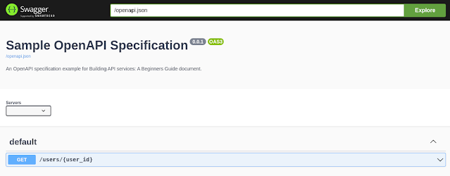
We can now access the UI http://127.0.0.1:8080/ui/ for an UI provided from Swagger about your REST API based on the specification.


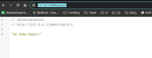
If we test it the API out using our path specified in our openapi.yaml, we can see the current autogenrated stub provides some dummy responses, and this part needs to be completed by us with our actual code and logic.


Implement your functionality on top of the generated server sub

As we mentioned ealier, you can find the default_controller.py file which shows your actual code and implemetation of your logic need to go based on the current stub that has been autogamically generated by the OpenAPI code generator.


def get_user(user_id):  # noqa: E501
    """get_user

    Gets a user # noqa: E501

    :param user_id: ID of a user
    :type user_id: str

    :rtype: Union[User, Tuple[User, int], Tuple[User, int, Dict[str, str]]
    """
    return 'do some magic!'

One thing to note is that the rtype (return type) is also very confusing here. It says Union or Tuple type but after many trials and errors, it turns out to be a JSON object - e.g., using json.dumps() - to be returned in order to work!

I hope you enjoyed the post and it is helpful for your REST API development journey!

SPARQL: FILTER NOT EXISTS and MINUS

I was wondering the difference between FILTER NOT EXISTS and MINUS, and found out a great answer here

The difference between FILTER NOT EXISTS and MINUS is related to the two styles of negation used by SPARQL. According to the specification:


The SPARQL query language incorporates two styles of negation, one based on filtering results depending on whether a graph pattern does or does not match in the context of the query solution being filtered, and one based on removing solutions related to another pattern.


Still according to the specification:


NOT EXISTS and MINUS represent two ways of thinking about negation, one based on testing whether a pattern exists in the data, given the bindings already determined by the query pattern, and one based on removing matches based on the evaluation of two patterns. In some cases they can produce different answers.


The two requests of your question are cited in the specification and the results are explained in the following way:


SELECT * {

   ?s ?p ?o .

   FILTER NOT EXISTS { ?x ?y ?z } .

}

This request evaluates to a result set with no solutions because { ?x ?y ?z } matches given any ?s ?p ?o, so NOT EXISTS { ?x ?y ?z } eliminates any solutions.


SELECT * {

   ?s ?p ?o .

   MINUS { ?x ?y ?z } .

}

In the request with MINUS, there is no shared variable between the first part (?s ?p ?o) and the second (?x ?y ?z) so no bindings are eliminated. 

AttributeError: module 'numpy.distutils.__config__' has no attribute 'blas_opt_info'

Errors

AttributeError: module 'numpy.distutils.__config__' has no attribute 'blas_opt_info'


Based on the issue discussed in https://github.com/numpy/numpy/issues/21079, a workaround is to change the cmodule in theano by commenting out the first line below and changing it to the second line.

$ vim ~/anaconda3/envs/pymc_env/lib/python3.10/site-packages/theano/link/c/cmodule.py:2621

2621             #blas_info = numpy.distutils.__config__.blas_opt_info
2622             blas_info = numpy.__config__.blas_opt_info

Variational Autoencoders

Autoencoder is an unsupervised model - a deep neural network architecture - which contains an encoder and decoder
  • The encoder component serves as compressing the input to a lower-dimensional representation;
  • The decoder aims to reconstruct the compressed representation back to the original input. 

The architecture is pretty simple, with the number of neurons in the layers of the encoder part (blue below) decreases, and then starts increasing again in the decoder part (purple below).

Input image => Dense(256) => Dense(64) => Dense(2) => Dense(64) => Dense(246) => Output (reconstructed image)

As one might expect, the loss is between the input image/data and reconstructed one, as the part of the name auto (self-supervised) implies.

Variational AutoEncoder (VAE) is the probablistic twist of the Autoencoder. Instead of giving deterministic output of both encoder and decoder in Autoencoder, that in VAE give probability distributions. 

As Autoencoder, the loss of VAE contains the reconstruction loss between the input data and reconstructed data. In addition, it also has a regularization term - the KL divergence between the posterior distribution (output of the encoder) and a prior (usually using a simple isotropic Gaussian). 

In this post, we go through the implementation of VAE with Tensorflow, Tensorflow Probability, and Keras. The example below is from Probabilistic Deep Learning with TensorFlow 2 course from Coursera, which by the way, I am highly recommend if you want to get familiar with Tensorflow Probability module. 

Contents


Import required packages


import tensorflow as tf
import tensorflow_probability as tfp
import seaborn as sns
import matplotlib
import numpy as np
import matplotlib.pyplot as plt

from tensorflow.keras.models import Sequential, Model
from tensorflow.keras.layers import Flatten, Dense, Reshape

print("tensorflow", tf.__version__)
print("tensorflow probability", tfp.__version__)
print("matplotlib", matplotlib.__version__)
print("numpy", np.__version__)
print("seaborn", sns.__version__)

tfd = tfp.distributions
tfpl = tfp.layers

tensorflow 2.8.0
tensorflow probability 0.14.0
matplotlib 3.8.0
numpy 1.26.0
seaborn 0.13.0


Fashion MNIST dataset

As we did in the Autoencoder post, we use the Fashion MNIST dataset is from Zalando. Zalando is a publicly traded German online retailer of shoes, fashion and beauty active across Europe. 

The dataset consists of a training set of 60,000 examples and a test set of 10,000 examples. Each example is a 28x28 grayscale image, associated with a label from 10 classes. We don't use those labels but only use images as we want to use Autoencoder to compress and reconstruct a given image. Let's get started.

# Fashion MNIST dataset

(X_train, y_train), (X_test, y_test) = tf.keras.datasets.fashion_mnist.load_data()

# If using Bernoulli, we can scale by simply dividing the max value 
#X_train = X_train.astype('float32')/256.
#X_test = X_test.astype('float32')/256.
# If we use Beta distribution defined within interval (0,1), 
# we need to scale images to the range (avoiding 0)
X_train = X_train.astype('float32')/256. + 0.5/256
X_test = X_test.astype('float32')/256. + 0.5/256

print(X_train.shape)

class_names = np.array([
    'T-shirt/top', 
    'Trouser/pants', 
    'Pullover shirt', 
    'Dress',
    'Coat', 
    'Sandal', 
    'Shirt', 
    'Sneaker', 
    'Bag',
    'Ankle boot'
])
(60000, 28, 28)

# Show some examples of the data

n_examples = 1000
example_images = X_test[0:n_examples]
example_labels = y_test[0:n_examples]

fig, axes = plt.subplots(1, 5, figsize=(15, 4))
for i in range(len(axes)):
    axes[i].imshow(example_images[i], cmap='binary')
    axes[i].set_title(class_names[example_labels[i]])
    axes[i].axis('off')


Encoder

The same as Autoencoder post, we keep the encoded dimention as 2, i.e., the output of the encoder is 2-dimentional vector - 2 random variables from probability distributions. And as mentioned earlier, we have a prior distribution for the KL divergence loss between it and the posterior distribution (the output distribution from encoder for those 2 random variables).

encoded_dim = 2

# Identity covariance matrix by default
prior = tfd.MultivariateNormalDiag(
    loc=tf.zeros(encoded_dim)
)

Here, we list three different versions for the encoder part. You can focus on first version only and then come back to investigate other versions if you are interested in learning more.

The posterior distribution is also multivariate Gaussian, but its parameters will be learned during training. The KLDivergenceAddLoss is a bypass layer, but will automatically add KL divergence loss between the prior and posterior to the main loss - the reconstruction loss.

# Encoder version 1
# Feel free to skip other versions and come back later

encoder = Sequential([
    Flatten(input_shape=(28, 28)),
    Dense(256, activation='relu'),
    Dense(64, activation='relu'),
    Dense(tfpl.MultivariateNormalTriL.params_size(encoded_dim)),
    tfpl.MultivariateNormalTriL(encoded_dim),
    tfpl.KLDivergenceAddLoss(prior)
])

print(encoder.losses, end='\n\n')
print(encoder(example_images), end='\n\n')
print(encoder.losses)

[tf.Tensor 'kl_divergence_add_loss_1/kldivergence_loss/batch_total_kl_divergence:0' shape=() dtype=float32]

tfp.distributions._TensorCoercible("sequential_2_multivariate_normal_tri_l_1_tensor_coercible", batch_shape=[1000], event_shape=[2], dtype=float32)

[tf.Tensor: shape=(), dtype=float32, numpy=0.89796853]

The second version gives more details of some parameters in the KLDivergenceAddLoss.

# Encoder version 2: with some arguments

encoder = Sequential([
    Flatten(input_shape=(28, 28)),
    Dense(256, activation='relu'),
    Dense(64, activation='relu'),
    Dense(tfpl.MultivariateNormalTriL.params_size(encoded_dim)),
    tfpl.MultivariateNormalTriL(encoded_dim),
    tfpl.KLDivergenceAddLoss(
        prior,
        use_exact_kl=False,
        weight=1.5,
        test_points_fn=lambda d: d.sample(10),
        test_points_reduce_axis=0
    )
])
  • weight: what multiple of KL divergence to be added to the loss, useful for implementing 𝛽-VAE, where 𝛽 indicates the weight of KL divergence.
  • test_points_fn: Receives batch of distributions, returns tensor of samples of shape (n_sample, batch_size, dim_z). These samples are converted to scalar value. $z_{ij}$ is the $i$-th sample for the observation $x_j$ (is at (i,j,:) in the tensor of samples) is mapped to $\log q(z_{ij})|x_j-\log p(z_{ij})$. This implies the tensor of samples returned by test_points_fn is converted into a tensor of values with a shape (n_samples, batch)
  • test_points_reduce_axis: to compute the loss added to the model, this arg indicates axis to average over (reduce_mean)
We can do exactly the same thing without using the KLDivergenceAddLoss. Instead, we can declare the KLDivergenceRegularizer as below and specify the activity_regularizer parameter in the MultivariateNormalTriL directly.

# Encoder version 3: Using KLDivergenceRegularizer

divergence_regularizer = tfpl.KLDivergenceRegularizer(
    prior,
    use_exact_kl=False,
    test_points_fn=lambda d: d.sample(10),
    test_points_reduce_axis=0
)

encoder = Sequential([
    Flatten(input_shape=(28, 28)),
    Dense(256, activation='relu'),
    Dense(64, activation='relu'),
    Dense(tfpl.MultivariateNormalTriL.params_size(encoded_dim)),
    tfpl.MultivariateNormalTriL(
        encoded_dim, 
        activity_regularizer=divergence_regularizer
    ),
])
We can first look at some encoded images before training. As one might expect, there is no clusters exhibit as the encoder is before any training.

pretrain_example_encodings = encoder(example_images).mean().numpy()

# Plot encoded examples before training 

f, ax = plt.subplots(1, 1, figsize=(7, 7))
sns.scatterplot(x=pretrain_example_encodings[:, 0],
                y=pretrain_example_encodings[:, 1],
                hue=class_names[example_labels], ax=ax,
                palette=sns.color_palette("colorblind", 10));
ax.set_xlabel('Encoding dimension 1'); ax.set_ylabel('Encoding dimension 2')
ax.set_title('Encodings of example images before training')


Decoder

For decoder part, we also use two different versions/options for modeling the output distribution. First one uses Bernoulli distribution and the second one uses Beta distribution. Tensorflow Probability provides an IndependentBernoulli layer which we can directly use for the first version. For the second one, as there is no such independent Beta layer implemented, we bake one from scratch using the DistributionLambda layer.

# Decoder version 1: Using IndependentBernoulli

decoder = Sequential([
    Dense(64, activation='relu', input_shape=(encoded_dim,)),
    Dense(256, activation='relu'),
    Dense(28*28),
    tfpl.IndependentBernoulli((28, 28))
])

# Decoder version 2: Using Independent Beta Distribution
# Since there is no IndependentBeta layer, bake one from scratch

decoder = Sequential([
    Dense(64, activation='relu', input_shape=(encoded_dim,)),
    Dense(256, activation='relu'),
    Dense(28*28*2, activation='exponential'), # non-nengative for Beta distribution params
    Reshape((28, 28, 2)),
    tfpl.DistributionLambda(
        lambda t: tfd.Independent(
            tfd.Beta(
                concentration1=t[..., 0],
                concentration0=t[..., 1]
            )
        )
    )
])

VAE

Finally, we use both encoder and decoder to build our VAE model. For the loss part, as we mentioned earlier, the KLDivergenceAddLoss layer already automatically add the KL/regularization loss to the main loss. Here we only need to specify the log loss.

vae = Model(
    inputs=encoder.inputs, 
    outputs=decoder(encoder.outputs)
)

def log_loss(x_true, p_x_given_z):
    return -tf.reduce_sum(p_x_given_z.log_prob(x_true))

vae.compile(loss=log_loss,)
vae.fit(
    x=X_train, 
    y=X_train,
    validation_data=(X_test, X_test),
    epochs=10,
    batch_size=32
)

WARNING:tensorflow:@custom_gradient grad_fn has 'variables' in signature, but no ResourceVariables were used on the forward pass.
1874/1875 [============================>.] - ETA: 0s - loss: -55572.9219WARNING:tensorflow:@custom_gradient grad_fn has 'variables' in signature, but no ResourceVariables were used on the forward pass.
WARNING:tensorflow:@custom_gradient grad_fn has 'variables' in signature, but no ResourceVariables were used on the forward pass.
1875/1875 [==============================] - 34s 16ms/step - loss: -55578.1367 - val_loss: -62465.1016
Epoch 2/10
1875/1875 [==============================] - 28s 15ms/step - loss: -64829.3750 - val_loss: -65042.4648
Epoch 3/10
1875/1875 [==============================] - 29s 15ms/step - loss: -67461.9844 - val_loss: -70393.7500
Epoch 4/10
1875/1875 [==============================] - 29s 15ms/step - loss: -69034.2734 - val_loss: -66066.8672
Epoch 5/10
1875/1875 [==============================] - 29s 15ms/step - loss: -70065.8438 - val_loss: -68278.2109
Epoch 6/10
1875/1875 [==============================] - 29s 15ms/step - loss: -70965.3438 - val_loss: -69826.4219
Epoch 7/10
1875/1875 [==============================] - 29s 15ms/step - loss: -71667.5000 - val_loss: -72257.3984
Epoch 8/10
1875/1875 [==============================] - 29s 15ms/step - loss: -72232.3594 - val_loss: -68337.1094
Epoch 9/10
1875/1875 [==============================] - 29s 16ms/step - loss: -72632.1641 - val_loss: -71673.4922
Epoch 10/10
1875/1875 [==============================] - 30s 16ms/step - loss: -72972.3281 - val_loss: -72791.6250

Results

First, we can plot some examples using the trained encoder this time.

# Generate an example reconstruction

example_reconstruction = vae(example_images).mean().numpy().squeeze()

# Plot the example reconstructions

fig, axs = plt.subplots(2, 6, figsize=(16, 5))

for j in range(6):
    axs[0, j].imshow(example_images[j, :, :].squeeze(), cmap='binary')
    axs[1, j].imshow(example_reconstruction[j, :, :], cmap='binary')
    axs[0, j].axis('off')
    axs[1, j].axis('off')

Finally, we can look at whether those encoded images exhibit some clusters after training. As we can observer from the right figure, some clusters can be found which contains images in the same or similar label.

# Compute example encodings after training

posttrain_example_encodings = encoder(example_images).mean().numpy()

# Compare the example encodings before and after training

f, axs = plt.subplots(nrows=1, ncols=2, figsize=(15, 7))
sns.scatterplot(
    x=pretrain_example_encodings[:, 0],
    y=pretrain_example_encodings[:, 1],
    hue=class_names[example_labels], ax=axs[0],
    palette=sns.color_palette("colorblind", 10)
)
sns.scatterplot(
    x=posttrain_example_encodings[:, 0],
    y=posttrain_example_encodings[:, 1],
    hue=class_names[example_labels], 
    ax=axs[1],
    palette=sns.color_palette("colorblind", 10)
)

axs[0].set_title('Encodings of example images before training');
axs[1].set_title('Encodings of example images after training');

for ax in axs: 
    ax.set_xlabel('Encoding dimension 1')
    ax.set_ylabel('Encoding dimension 2')
    ax.legend(loc='upper right')


In this post, we introduced Variational AutoEncoder, which is the probablistic twist of Autoencoder. In contrast to the Autoencoder, it is designed or trained to generate images, and it is not deterministic as the Autoencoder (the output of encoder and decoder given an input image). For example, VAE allows sampling from the distributions in the encoder and decoder and will lead to different results for a given image.

403 Forbidden errors when request a webpage using Python requests

Error 

403 Forbidden errors when request a web page using Python requests. 


Cause

Usually, this is caused by the lack of headers indicating User-Agent. We can add the header information with User-Agent and send the request again.

import requests

url = 'http://example.com/'

headers = {'User-Agent': 'Mozilla/5.0 (Macintosh; Intel Mac OS X 10_11_5) AppleWebKit/537.36 (KHTML, like Gecko) Chrome/50.0.2661.102 Safari/537.36'}

result = requests.get(url, headers=headers)
# Check the status code 
print(result.status_code)

WARNING:tensorflow:Early stopping conditioned on metric `val_loss` which is not available. Available metrics are: xxx

Error message 

"WARNING:tensorflow:Early stopping conditioned on metric `val_loss` which is not available. Available metrics are: loss,mae,mse,mape"


Cause

This is normally due to the validation dataset is empty, so there is no associated val_loss for the empty validation data.

Preparing windowed dataset for time series forecasting


Windowed dataset is required in many forecasting methods, especially for machine learning-based approaches. As an example, given a time series, e.g., [1,3,5,7,9], and a window size of 2, the corresponding windowed dataset could be as follows, which can be used for training a machine learning model where each element in X represents windowed data while each element in y represents a corresponding label/target/next value to be predicted.

X = [[1,3], [3,5], [5,7]]
y = [[5], [7], [9]]

Importing packages


import tensorflow as tf
import numpy as np

print(tf.__version__)
print(np.__version__)

2.4.1
1.19.2  


For simplicity, here we create a sequence of numbers as our example time series data.


ts = np.arange(1, 100, 2)

array([ 1, 3, 5, 7, 9, 11, 13, 15, 17, 19, 21, 23, 25, 27, 29, 31, 33, 35, 37, 39, 41, 43, 45, 47, 49, 51, 53, 55, 57, 59, 61, 63, 65, 67, 69, 71, 73, 75, 77, 79, 81, 83, 85, 87, 89, 91, 93, 95, 97, 99])


Implementation

The window_dataset() below provides a functionality to produce the windowed dataset for a given time series (ts) and the window_size. We delve into some details of the code in the following.


def window_dataset(ts, window_size=2):
    """ Process the time series into windowed dataset 
    
    :parameter ts: time series data
    
    Return data, targets where data and targets are both list
        each element in data is history in a window, 
        each element in targets is the next value
    """
    data = list()
    targets = list()
    
    dataset = tf.data.Dataset.from_tensor_slices(ts)
    dataset = dataset.window(
        window_size+1, 
        shift=1, 
        drop_remainder=True
    )
    dataset = dataset.flat_map(lambda w: w.batch(window_size+1))
    dataset = dataset.map(lambda w: (w[:-1], w[-1:]))
    
    for (x, y) in dataset.as_numpy_iterator():
        data.append(x)
        targets.append(y)
        
    return data, targets


data, targets = window_dataset(ts)

for x,y in zip(data, targets):
    print(x,y)

[1 3] [5]
[3 5] [7]
[5 7] [9]
[7 9] [11]
[ 9 11] [13]
[11 13] [15]
[13 15] [17]
[15 17] [19]
[17 19] [21]
[19 21] [23]
[21 23] [25]
[23 25] [27]
[25 27] [29]
[27 29] [31]
[29 31] [33]
[31 33] [35]
[33 35] [37]
[35 37] [39]
[37 39] [41]
[39 41] [43]
[41 43] [45]
[43 45] [47]
[45 47] [49]
[47 49] [51]
[49 51] [53]
[51 53] [55]
[53 55] [57]
[55 57] [59]
[57 59] [61]
[59 61] [63]
[61 63] [65]
[63 65] [67]
[65 67] [69]
[67 69] [71]
[69 71] [73]
[71 73] [75]
[73 75] [77]
[75 77] [79]
[77 79] [81]
[79 81] [83]
[81 83] [85]
[83 85] [87]
[85 87] [89]
[87 89] [91]
[89 91] [93]
[91 93] [95]
[93 95] [97]
[95 97] [99]

Given the windowed dataset, we can fit any forecasting model. Here, we simply use a linear regression to fit the windowed dataset for illustration.

from sklearn.linear_model import LinearRegression

model = LinearRegression(fit_intercept=True)
model.fit(data, targets)
model.predict([[97,99]])

array([[101.]])


Details

Now, we move on to some details of the window_dataset() method. First step is creating a Tensorflow dataset. The from_tensor_slices(ts) creates a Dataset whose elements are slices of the given tensors.


dataset = tf.data.Dataset.from_tensor_slices(ts)
for d in dataset:
    print(d)
    break

tf.Tensor(1, shape=(), dtype=int64)


The Tensorflow dataset provides a method - window() - which a dataset of "windows". According to the documentation, each "window" is a dataset that contains a subset of elements of the input dataset. These are finite datasets of size size (or possibly fewer if there are not enough input elements to fill the window and drop_remainder evaluates to False). As the subset is still a dataset, we use list() and as_numpy_iterator() which returns an iterator which converts all elements of the dataset to numpy.


window_size = 2
dataset = dataset.window(
    window_size+1, 
    shift=1, 
    drop_remainder=True
)
for d in dataset:
    # Each d will be sub-dataset of the dataset
    print(list(d.as_numpy_iterator()))
    break

[1, 3, 5]


Here, we grab all data in each sub-dataset and flattens the result.


# Maps .batch across each sub-dataset
dataset = dataset.flat_map(lambda w: w.batch(window_size+1))
for d in dataset:
    print(d)
    break

tf.Tensor([1 3 5], shape=(3,), dtype=int64)


Finally, we split the data part and target one for each element in the dataset, and each pair will be a training example for training a forecasting model.


dataset = dataset.map(lambda w: (w[:-1], w[-1:]))
for (x, y) in dataset.as_numpy_iterator():
    print(x, y)
    break

[1 3] [5]
That's it for preparing windowed dataset for time series forecasting. Although we used Tensorflow to implement the preprocessing step, you can also try to use other ways to implement the same functionality as long as you can derive the same output.

Autoencoders

Autoencoder is an unsupervised model - a deep neural network architecture - which contains an encoder and decoder. The encoder component serves as compressing the input to a lower-dimensional representation while the decoder aims to reconstruct the compressed representation back to the original input. 

The architecture is pretty simple, with the number of neurons in the layers of the encoder part (blue below) decreases, and then starts increasing again in the decoder part (purple below).

Input image => Dense(256) => Dense(64) => Dense(2) => Dense(64) => Dense(246) => Output (reconstructed image)

As one might expect, the loss is between the input image/data and reconstructed one, as the part of the name auto (self-supervised) implies.

In this post, we go through the implementation of Autoencoder with Tensorflow and Keras. The example below is from Probabilistic Deep Learning with TensorFlow 2 course from Coursera, which by the way, I am highly recommend if you want to get familiar with Tensorflow Probability module. However, for Autoencoder, we don't necessarily need the Tensorflow Probability module (The module is useful when implementing Variational AutoEncoder, a generative variant of Autoencoder). 

Contents

  • Import required packages
  • Fashion MNIST dataset
  • Encoder
  • Decoder
  • Encoding results after training
  • Autoencoder reconstructed results
  • Import required packages

    
    import tensorflow
    import matplotlib
    import seaborn as sns
    import numpy as np
    import matplotlib.pyplot as plt
    
    from tensorflow.keras.models import Sequential, Model
    from tensorflow.keras.layers import Dense, Flatten, Reshape
    
    print(tensorflow.__version__)
    print(matplotlib.__version__)
    print(np.__version__)
    print(sns.__version__)
    print(matplotlib.__version__)
    
    
    2.1.0
    3.0.3
    1.18.3
    0.9.0
    3.0.3

    Fashion MNIST dataset

    Fashion MNIST dataset is from Zalando - a publicly traded German online retailer of shoes, fashion and beauty active across Europe. The dataset consists of a training set of 60,000 examples and a test set of 10,000 examples. Each example is a 28x28 grayscale image, associated with a label from 10 classes. We don't use those labels but only use images as we want to use Autoencoder to compress and reconstruct a given image. Let's get started.
    
    # Load Fashion MNIST
    
    (x_train, y_train), (x_test, y_test) = tf.keras.datasets.fashion_mnist.load_data()
    x_train = x_train.astype('float32')/255.
    x_test = x_test.astype('float32')/255.
    class_names = np.array([
        'T-shirt/top', 
        'Trouser/pants', 
        'Pullover shirt', 
        'Dress',
        'Coat', 
        'Sandal', 
        'Shirt', 
        'Sneaker', 
        'Bag',
        'Ankle boot'
    ])
    
    print(x_train.shape)
    
    
    (60000, 28, 28)

    We can have a look on some of those images.

    
    # Display a few examples
    
    n_examples = 1000
    example_images = x_test[0:n_examples]
    example_labels = y_test[0:n_examples]
    
    f, axs = plt.subplots(1, 5, figsize=(15, 4))
    for j in range(len(axs)):
        axs[j].imshow(example_images[j], cmap='binary')
        axs[j].axis('off')


    Encoder

    Now we move on to the implementation of the encoder part of Autoencoder. The encoder simply flattens the input image and goes through two Dense layers followed by another Dense layer with desired encoding dimensionality, which is 2 here.

    We can check the compressed or encoded images using this encoder. Note as the encoder has not been trained yet, we should see those encoded images from different class are not distinguishable in the encoding space.

    
    # Define the encoder
    
    encoded_dim = 2
    encoder = Sequential([
        Flatten(input_shape=(28, 28)),
        Dense(256, activation='sigmoid'),
        Dense(64, activation='sigmoid'),
        Dense(encoded_dim)
    ])
    
    # Encode examples before training
    
    pretrain_example_encodings = encoder(example_images).numpy()
    
    # Plot encoded examples before training 
    
    f, ax = plt.subplots(1, 1, figsize=(7, 7))
    sns.scatterplot(pretrain_example_encodings[:, 0],
                    pretrain_example_encodings[:, 1],
                    hue=class_names[example_labels], ax=ax,
                    palette=sns.color_palette("colorblind", 10));
    ax.set_xlabel('Encoding dimension 1'); ax.set_ylabel('Encoding dimension 2')
    ax.set_title('Encodings of example images before training');


    Decoder

    Given the 2-dim encoded images, the decoder part tries to reconstruct the input image. And we can use the encoder and deconder that we've just defined to define the Autoencoder. Afterwards, we compile and fit the model as we usually do for training the Autoencoder.
    
    # Define the decoder
    
    decoder = Sequential([
        Dense(64, activation='sigmoid', input_shape=(encoded_dim,)),
        Dense(256, activation='sigmoid'),
        Dense(28*28, activation='sigmoid'),
        Reshape((28, 28))
    ])
    
    # Compile and fit the model
    
    autoencoder = Model(
        inputs=encoder.input,
        outputs=decoder(encoder.output)
    )
    
    # Specify loss - input and output is in [0., 1.], so we can use a binary cross-entropy loss
    autoencoder.compile(loss='binary_crossentropy')
    
    # Fit model - highlight that labels and input are the same
    autoencoder.fit(
        x=x_train, 
        y=x_train,
        epochs=10,
        batch_size=32
    )
    
    Train on 60000 samples
    Epoch 1/10 60000/60000 [==============================] - 76s 1ms/sample - loss: 0.4078
    Epoch 2/10 60000/60000 [==============================] - 74s 1ms/sample - loss: 0.3510
    Epoch 3/10 60000/60000 [==============================] - 75s 1ms/sample - loss: 0.3395
    Epoch 4/10 60000/60000 [==============================] - 78s 1ms/sample - loss: 0.3342
    Epoch 5/10 60000/60000 [==============================] - 78s 1ms/sample - loss: 0.3308
    Epoch 6/10 60000/60000 [==============================] - 78s 1ms/sample - loss: 0.3284
    Epoch 7/10 60000/60000 [==============================] - 77s 1ms/sample - loss: 0.3264
    Epoch 8/10 60000/60000 [==============================] - 74s 1ms/sample - loss: 0.3248
    Epoch 9/10 60000/60000 [==============================] - 70s 1ms/sample - loss: 0.3234
    Epoch 10/10 60000/60000 [==============================] - 84s 1ms/sample - loss: 0.3226

    Encoding results after training

    Now the Autoencoder has been trained. We can again check the encoded/compressed images to see if those encoded/compressed representations of images exhibit some interesting patterns ideally according to their categories.
    
    # Compute example encodings after training
    
    posttrain_example_encodings = encoder(example_images).numpy()
    
    # Compare the example encodings before and after training
    
    f, axs = plt.subplots(nrows=1, ncols=2, figsize=(15, 7))
    sns.scatterplot(pretrain_example_encodings[:, 0],
                    pretrain_example_encodings[:, 1],
                    hue=class_names[example_labels], ax=axs[0],
                    palette=sns.color_palette("colorblind", 10));
    sns.scatterplot(posttrain_example_encodings[:, 0],
                    posttrain_example_encodings[:, 1],
                    hue=class_names[example_labels], ax=axs[1],
                    palette=sns.color_palette("colorblind", 10));
    
    axs[0].set_title('Encodings of example images before training');
    axs[1].set_title('Encodings of example images after training');
    
    for ax in axs: 
        ax.set_xlabel('Encoding dimension 1')
        ax.set_ylabel('Encoding dimension 2')
        ax.legend(loc='upper right')


    As we can see from the figure, after training, images belong to the same or similar categories such as "Ankle boot" and "Sneaker" tend to be clustered together.

    Autoencoder reconstructed results

    Here we can reconstruct some images using the trained Autoencoder, which shows the reconstructed images are reasonably close to the given images.
    
    # Compute the autoencoder's reconstructions
    
    reconstructed_example_images = autoencoder(example_images)
    
    # Evaluate the autoencoder's reconstructions
    
    f, axs = plt.subplots(2, 5, figsize=(15, 4))
    for j in range(5):
        axs[0, j].imshow(example_images[j], cmap='binary')
        axs[1, j].imshow(reconstructed_example_images[j].numpy().squeeze(), cmap='binary')
        axs[0, j].axis('off')
        axs[1, j].axis('off')


    In this post, we introduced Autoencoder, which trains the encoder and decoder parts via "self-supervised" way by minimizing the reconstruction loss. Although Autoencoder can be useful for compression and reconstruction, it is not designed or trained to generate images. VAE (Variational Autoencoder) is the probablistic twist of Autoencoder for that purpose, which we will look into in another post.

    TypeError: Descriptors cannot not be created directly.

    TypeError: Descriptors cannot not be created directly.

    If this call came from a _pb2.py file, your generated code is out of date and must be regenerated with protoc >= 3.19.0.

    If you cannot immediately regenerate your protos, some other possible workarounds are:

     1. Downgrade the protobuf package to 3.20.x or lower.

     2. Set PROTOCOL_BUFFERS_PYTHON_IMPLEMENTATION=python (but this will use pure-Python parsing and will be much slower).  

    ####################################################


    As suggested by the error message itself, we just need to downgrade the protobuf package to 3.20.x or lower.

    $ pip install protobuf==3.20.*

    TypeError: Descriptors cannot not be created directly.

     2023-10-19 10:01:41.895250: W tensorflow/stream_executor/platform/default/dso_loader.cc:64] Could not load dynamic library 'libcudart.so.11.0'; dlerror: libcudart.so.11.0: cannot open shared object file: No such file or directory

    2023-10-19 10:01:41.895278: I tensorflow/stream_executor/cuda/cudart_stub.cc:29] Ignore above cudart dlerror if you do not have a GPU set up on your machine.

    Traceback (most recent call last):

      File "t01.py", line 7, in <module>

        import tensorflow.compat.v2 as tf

      File "/home/parklize/Documents/code/tfp/venv/lib/python3.8/site-packages/tensorflow/__init__.py", line 37, in <module>

        from tensorflow.python.tools import module_util as _module_util

      File "/home/parklize/Documents/code/tfp/venv/lib/python3.8/site-packages/tensorflow/python/__init__.py", line 37, in <module>

        from tensorflow.python.eager import context

      File "/home/parklize/Documents/code/tfp/venv/lib/python3.8/site-packages/tensorflow/python/eager/context.py", line 29, in <module>

        from tensorflow.core.framework import function_pb2

      File "/home/parklize/Documents/code/tfp/venv/lib/python3.8/site-packages/tensorflow/core/framework/function_pb2.py", line 16, in <module>

        from tensorflow.core.framework import attr_value_pb2 as tensorflow_dot_core_dot_framework_dot_attr__value__pb2

      File "/home/parklize/Documents/code/tfp/venv/lib/python3.8/site-packages/tensorflow/core/framework/attr_value_pb2.py", line 16, in <module>

        from tensorflow.core.framework import tensor_pb2 as tensorflow_dot_core_dot_framework_dot_tensor__pb2

      File "/home/parklize/Documents/code/tfp/venv/lib/python3.8/site-packages/tensorflow/core/framework/tensor_pb2.py", line 16, in <module>

        from tensorflow.core.framework import resource_handle_pb2 as tensorflow_dot_core_dot_framework_dot_resource__handle__pb2

      File "/home/parklize/Documents/code/tfp/venv/lib/python3.8/site-packages/tensorflow/core/framework/resource_handle_pb2.py", line 16, in <module>

        from tensorflow.core.framework import tensor_shape_pb2 as tensorflow_dot_core_dot_framework_dot_tensor__shape__pb2

      File "/home/parklize/Documents/code/tfp/venv/lib/python3.8/site-packages/tensorflow/core/framework/tensor_shape_pb2.py", line 36, in <module>

        _descriptor.FieldDescriptor(

      File "/home/parklize/Documents/code/tfp/venv/lib/python3.8/site-packages/google/protobuf/descriptor.py", line 561, in __new__

        _message.Message._CheckCalledFromGeneratedFile()

    TypeError: Descriptors cannot not be created directly.

    If this call came from a _pb2.py file, your generated code is out of date and must be regenerated with protoc >= 3.19.0.

    If you cannot immediately regenerate your protos, some other possible workarounds are:

     1. Downgrade the protobuf package to 3.20.x or lower.

     2. Set PROTOCOL_BUFFERS_PYTHON_IMPLEMENTATION=python (but this will use pure-Python parsing and will be much slower).


    More information: https://developers.google.com/protocol-buffers/docs/news/2022-05-06#python-updates

    =======================================
    To solve the issue, I needed to downgrade protobuf using pip
    $ pip install protobuf==3.20.*

    Note: the * above is not to be taken literally, it's called a "wildcard". You put your own number in there as needed, as in 3.20.1, 3.20.5, etc. See https://stackoverflow.com/questions/72899948/how-to-downgrade-protobuf for details.

    I/O exception(java.io.IOException)caught when processing request to{}->tcp://localhost:2376 xxx in Ubuntu

    The error occurred when I'm following in28minutes's course - "Microservices" on Udemy. When using maven build command "spring-boot:build-image -DskipTest" to create a Docker image, it gives the error. After digging a while, I found out that the default one is a socket without TCP on Ubuntu.

    I had to allow Docker to accept requests from remote hosts by configuring it to listen on an IP address and port as well as the UNIX socket following steps from here.


    1.Edit the docker.service file.

    sudo systemctl edit docker.service
    

    Lets say we want to listen for connections from any remote host on port 2376

    2. we need to add this lines:

    [Service]
    ExecStart=
    ExecStart=/usr/bin/dockerd -H fd:// -H tcp://0.0.0.0:2376
    

    3. Write the changes (ctrl-o) and exit (ctrl-x).

    4. Reload the systemctl configuration.

    sudo systemctl daemon-reload
    

    5. Restart the Docker service.

    sudo systemctl restart docker.service
    

    6. Verify the dockerd daemon listening on the configured port using the netstat command.

    sudo netstat -lntp | grep dockerd
    

    here is the sequence:

    Also I needed to run the created Docker image with sudo. Another one usefule is creating symlink: sudo ln -s -f /home/[yourusername]/.docker/desktop/docker.sock /var/run/docker.sock

    Installing docker, getting: `PreDepends: init-system-helpers (>= 1.54~) but 1.51 is to be installed`

    •  wget http://ftp.kr.debian.org/debian/pool/main/i/init-system-helpers/init-system-helpers_1.60_all.deb
    • sudo apt install ./init-system-helpers_1.60_all.deb
    • And finally sudo apt install ./docker-desktop-*-amd64.deb

    How to decide the sample size of A/B testing using Python?

    Deciding the sample size for running A/B testing is an essential step. In this post, we take an example from the Udecity course - Overview of A/B Testing. 

    We are interested in changing the color of "Start Now" button on an Udecity-like website to see the effect of click-through probability, which is measured by 

    # of users clicked / # of users visited

    Based on 1000 users visited, we found that 100 users clicked. This gives us 10% of the click-through probability. We are also interested in 
    • significant level (usually referred as $\alpha$) of 5% (0.05)
    • practical significance level of 2%, i.e., minimum effect that we care about
    • power/sensitivity of 80% (fairly standard)

    First, we use an online calculator that has been introduced in the course: https://www.evanmiller.org/ab-testing/sample-size.html. The terminologies used by this calculator and the corresponding ones that we mentioned above are:
    • base conversion rate: click-through probability. This is estimated click-through probability before making the change
    • minimum detectable effect: practical significance level, and we care about absolute difference.
    • statistical power: power/sensitivity
    • significant level: significant level
    And the result of the calculator is 3,623.


    Here we use the same equation in Python to derive the same result mentioned above.


    ## Calculate required sample size
    def calc_sample_size(alpha, power, p, pct_mde, absolute=True):
        """ Based on https://www.evanmiller.org/ab-testing/sample-size.html
    
        Args:
            alpha (float): How often are you willing to accept a Type I error (false positive)?
            power (float): How often do you want to correctly detect a true positive (1-beta)?
            p (float): Base conversion rate
            pct_mde (float): Minimum detectable effect, relative to base conversion rate.
    
        """
        if absolute:
            delta = pct_mde
        else:
            delta = p*pct_mde
        t_alpha2 = norm.ppf(1.0-alpha/2)
        t_beta = norm.ppf(power)
    
        sd1 = np.sqrt(2 * p * (1.0 - p))
        sd2 = np.sqrt(p * (1.0 - p) + (p + delta) * (1.0 - p - delta))
    
        return int(np.ceil((t_alpha2 * sd1 + t_beta * sd2) * (t_alpha2 * sd1 + t_beta * sd2) / (delta * delta)))
    
    print(calc_sample_size(alpha=0.05, power=0.8, p=0.1, pct_mde=0.02))
    
    Output:
    3623
    
    As we can see, the Python method produces the same result as the online calculator.